 Akash Manohar John
Cosine Similarity
I found this tweet by @helloiamleonie at 5am while doom scrolling Twitter in bed. I looked up “cosine similarity” out of curiosity and that is what started it all for me, and hopefully for anyone reading this too.
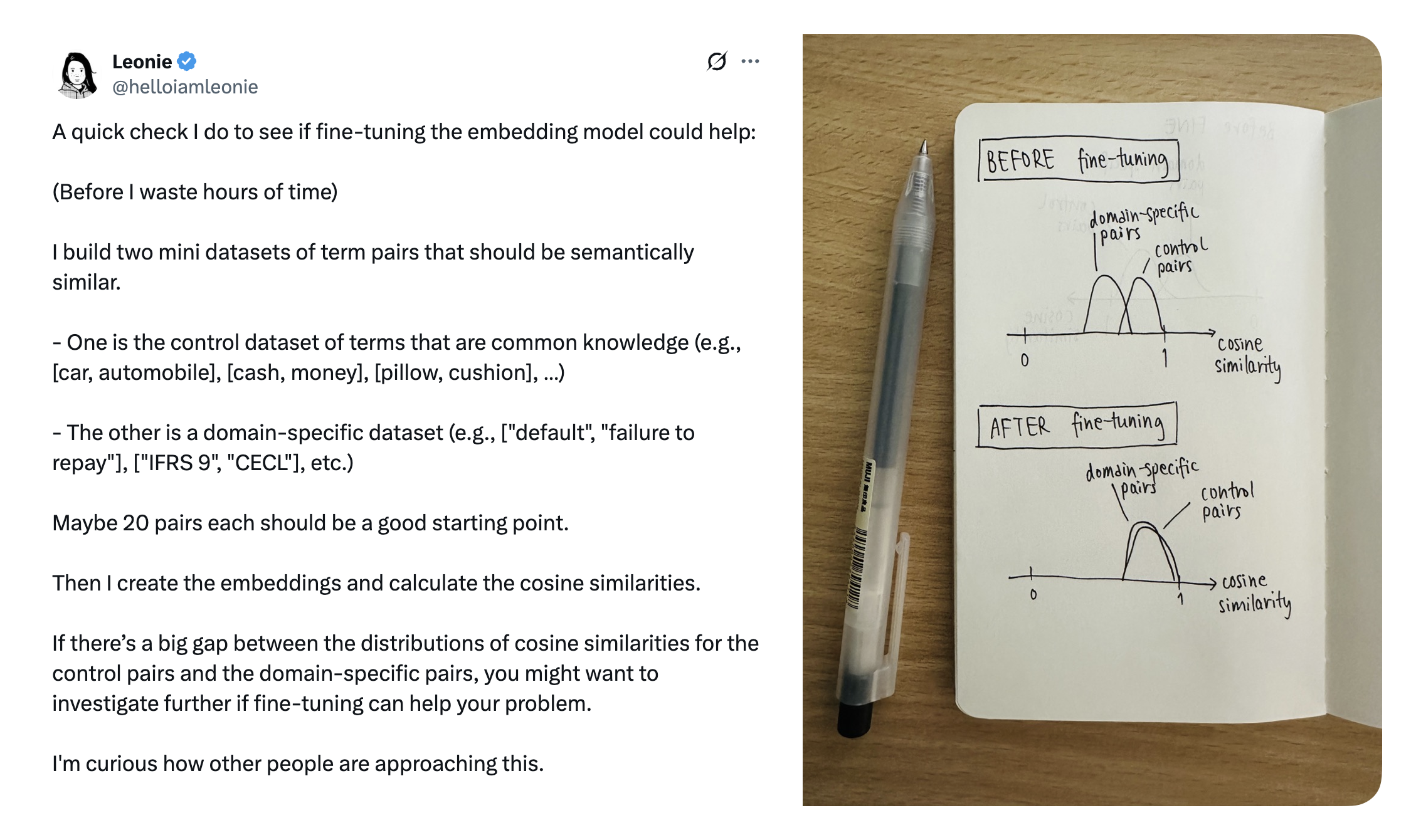
Source - https://x.com/helloiamleonie/status/1924758338966802709
Prerequisites
Lets get the prereqs out of the way first. Ensure numpy and openai libraries are installed and import them.
# Install packages
# !pip install openai python-dotenv numpy matplotlib
# Load environment vars from .env file.
# We have OPENAI_API_KEY in .env
from dotenv import load_dotenv
load_dotenv()

from openai import OpenAI
import numpy as np

# import this to plot some stuff
import matplotlib.pyplot as plt

# Create an OpenAI client, because we will be using this a few times
openai_client = OpenAI()
Comparison, beyond equality and regex
Given these phrases,
- A: “Pizza was delicious”
- B: “I loved the pizza”
- C: “The staff were extremely helpful”
In your code, if you were to check if these user reviews of a hotel are talking about the same thing, any possibility of using regex and equality is out of the window given the numerous things that customers can talk about. Cosine similarity helps your app understand that A & B are talking about similar things, and that C talks about something else entirely.
To start, we use a text embedding model to give us numbers that represent these sentences.
“Embedding” is a representation of data as an vector. For any given input, an embedding model returns a vector that represents a that piece of input. For a while, we’ll be using vector and embedding interchangeably.
Make a call to OpenAI, with the sentences as input. To keep things simple, we will ask for vectors of just two dimensions.
sentences = [
    "Pizza was delicious",
    "I loved the pizza",
    "The staff were extremely helpful"
]

# Fetch the embeddings
response = openai_client.embeddings.create(
    model="text-embedding-3-small",
    input=sentences,
    dimensions=2
)

# This loops through the response and collects the embedding vector for each sentence
sentence_vectors = [np.array(result.embedding) for result in response.data]

for sentence, vector in zip(sentences, sentence_vectors):
    print(f"Sentence: {sentence}")
    print(f"\t{vector[0]}, {vector[1]}\n")
This gives us these two-dimensional vectors:
| Sentence | Vector |
|---|---|
| Pizza was delicious | [-0.48245808482170105, -0.8759190440177917] |
| I loved the pizza | [0.1533546894788742, -0.9881712198257446] |
| The staff were extremely helpful | [-0.19024261832237244, 0.9817371368408203] |
We added another sentence “Pizza is bad” to find the vectors for. We will use this soon.
Plot the vectors to compare them
It’s hard to compare these vectors just by looking at them. So lets plot them on a graph.
import matplotlib.pyplot as plt

# plot the vectors
plot_vectors = np.array(sentence_vectors)
origin = np.zeros((3, 2))

# Create plot
fig, ax = plt.subplots()

# Plot vectors
ax.quiver(origin[:, 0], origin[:, 1], plot_vectors[:, 0], plot_vectors[:, 1],
          angles='xy', scale_units='xy', scale=1, color=['r', 'g', 'b'])

# Label each vector near its tip
labels = ['A', 'B', 'C']
for vec, label in zip(plot_vectors, labels):
    ax.text(vec[0]*1.05, vec[1]*1.05, label, fontsize=12)

# Axes setup
ax.set_aspect('equal')
ax.set_xlim(-3, 3)
ax.set_ylim(-3, 3)

# Move axes to origin
ax.spines['left'].set_position('zero')
ax.spines['bottom'].set_position('zero')
ax.spines['top'].set_color('none')
ax.spines['right'].set_color('none')

# Grid and title
ax.grid(True)
plt.title("Labeled Vectors with Axes at Origin")
plt.show()
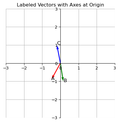
Notice A and B are close by. But C is pointing in an entirely different direction. Cosine similarity helps check how “similar” these vectors are. We will use the following function to calculate cosine similarity.
Copy-pasta this for now. We will explore this function later.
def cosine_similarity(vec1, vec2):
    vec1 = np.array(vec1)
    vec2 = np.array(vec2)
    dot_product = np.dot(vec1, vec2)
    norm_product = np.linalg.norm(vec1) * np.linalg.norm(vec2)
    return dot_product / norm_product
Let us compare the following sentences using cosine similarity:
- A: “Pizza was delicious”
- B: “I loved the pizza”
cosine_similarity(sentence_vectors[0], sentence_vectors[1])
This returns 0.7915707820894159.
Now compare A & C:
- A: “Pizza was delicious”
- C: “The staff were extremely helpful”
cosine_similarity(sentence_vectors[0], sentence_vectors[2])
This returns -0.7681381516634945.
Defining a range to decide if these numbers mean the inputs are similar or disimilar, is entirely upto your application. You may define that 0.7 is a good enough minimum score to indicate similarity.
Reasons behind choosing cosine similarity
Given two lines, A & B, that both start at the origin (0, 0), visually, it is easy to compare if they are pointing in the same direction (or atleast how close they are). If you had to translate this to code, geometry has the answer.
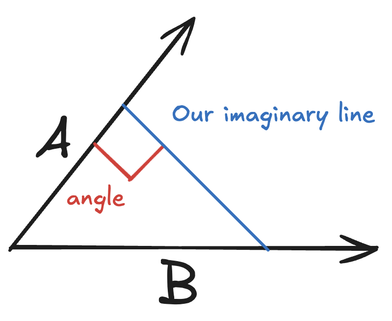
We are going to need another imaginary line. Pick any point on the line A, and draw a perpendicular line to the line B.
Now with our imaginary line in place, we get to use Pythagoras theorem since the angle between A and the imaginary line is 90 degrees. We can then use any equation that gives us a value to compare how close these lines are.
Inputs we have:
- A forms the adjacent side
- B is the hypotenuse
From trigonometry, if you remember “SOH CAH TOA”, the CAH is
cos = adj / hyp
Now we can use cos($\theta$) to decide if A and B are pointing in the same direction.
But why cosine? Why not sine, or tangent?
Bounded values
Are 50 and 55 close? Yes? What if the range was always betwen 50 and 55? Now the 50 and 55 seem like extremes.
Without bounds, a score to compare similarity is meaningless. Cosine always returns a value between -1 and +1. So now you can set your own definition of similarity. Lets say that you configure your app that any value between 0.7 and 1.0 means that the inputs are similar.
This disqualifies tan($\theta$), because has a much larger range -infinity to +infinity.
Ability to represent the entire range of values
When comparing vectors, our similarity test may result in any of the following:
- The inputs are similar
- The inputs are opposites
- The inputs are unrelated
So we need a function that can represent 3 distinct states. This immediately disqualifies sine. Because sin(0°) and sin(180°) have the same value even though the lines would point in the opposite directions.
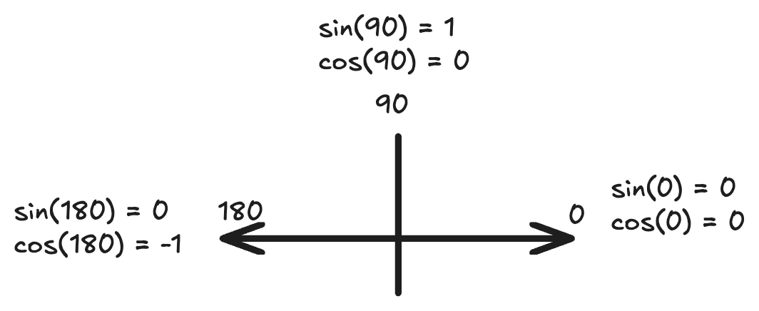
With cosine, we get:
- 1 if the input vectors are related - pointing in the same direction.
- 0 if the input vectors are unrelated (perpendicular).
- -1 if the input vectors are pointing in opposite directions (Example: “pizza is good” vs “pizza is bad”)
“Pizza is good” and “Pizza is bad” being opposites depends on the model’s understanding. But for now, we will assume that it understands pizzas and taste.
So cosine wins, atleast for this lesson.
Our cosine similarity function has been a black box so far. Next, we explore how to calculate cosine similarity, and also explore other functions to calculate similarity.